page under construction

Introduction

Impulse excitation, also known as impact excitation and resonance technique (see also Wikipedia), is a commonly used method to assess the stiffness of wood (and other materials) in both scientific and industrial settings. One or more modes of vibration are excited by a brief mechanical impulse, and their resonant frequencies measured. When combined with measurements of density and dimensions, these frequencies can be used to calculate elastic moduli – most commonly modulus of elasticity parallel to grain, which is an important property for construction timber. The technique may also be used to assess damping, which is an important property for wood used in musical instruments.

On this page, we will give some brief instructions on how to use this technique, with some provided functions for free Open Source statistical computing software R. The R code makes use of R packages seewave and tuneR. For a simple user interface, we recommend you use R with R-studio. If you already know how to use both R and the impact excitation method, you can go directly to our github “TimbR”project page to download the R-scripts.

The impulse excitation method

This is a non-destructive material characterisation technique in which an elastic solid is lightly struck with a hammer or projectile, giving it energy to vibrate at its natural frequencies. The induced vibration response, resulting from this momentary impulse, is measured with a suitable transducer such as a microphone, piezoelectric sensor, laser vibrometer or accelerometer. The acquired vibration signal in the time domain is converted to the frequency domain to determine the modal frequencies. If the shape is suitable (e.g. rectangular bars, cylindrical rods) these frequency spectra peaks can be used with geometry and mass measurements to calculate Young’s modulus, shear modulus, Poisson’s ratio and internal friction.

Several industrial machines use this “resonance” technique to measure timber stiffness for grading structural timber and assessing logs. We have made use of a fibre-gen ‘HITMAN’ HM200 and a Brookhuis MTG 960 series in our research for a number of years.

If the frequency of vibration is within the range of human hearing (~20 Hz to ~20 kHz), which is commonly the case for wood, then the measurement can be made with a simple audio microphone. This means the technique is very quick, simple and cheap to use. That said, we are not providing TimbR as a replacement for any specialist software or equipment (such as the Bing system by Cirad intended specifically for use with wood, or the Buzz-o-Sonic system from BuzzMac, and the long in use GrindoSonic from JW Lemmens), but rather as a learning tool, and entry level option for new and occasional users of the impulse excitation technique.

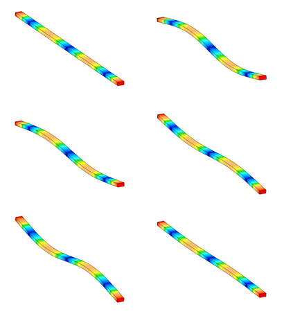
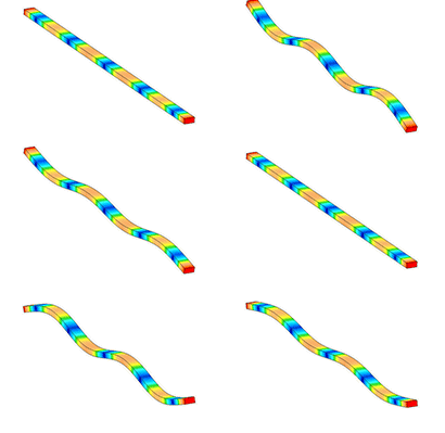
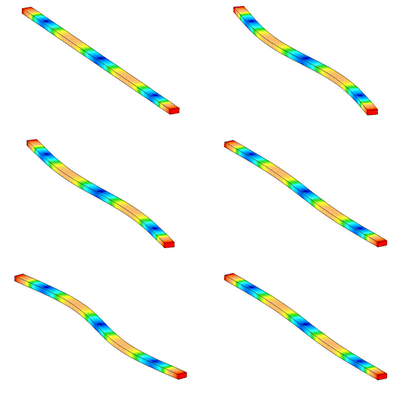
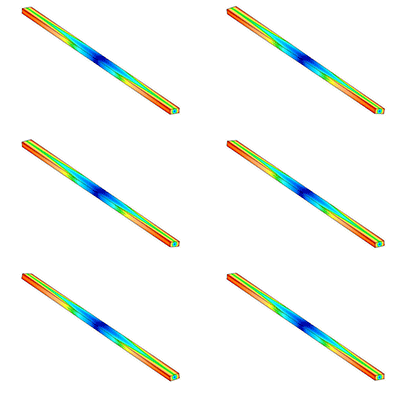
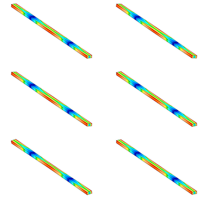
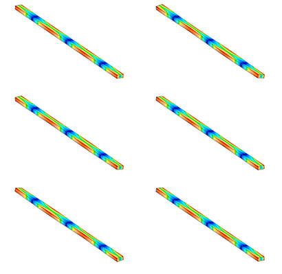
The most useful modes of free-free vibration for rectangular sawn timber are: longitudinal, flexural and torsional


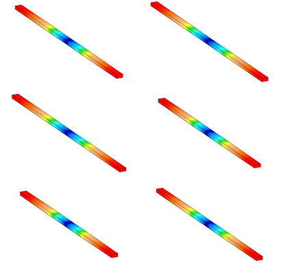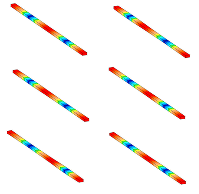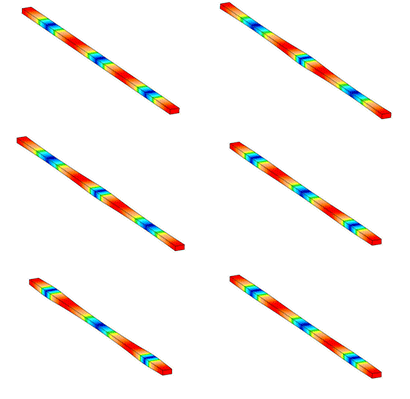1st longitudinal	2nd longitudinal	3rd longitudinal

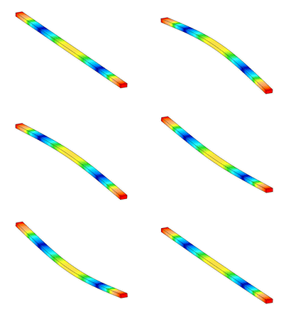1st flexural minor	2nd flexural minor	3rd flexural minor

1st flexural major	2nd flexural major

1st torsional	2nd torsional	3rd torsional

We might call the longitudinal and torsional modes harmonics because the frequencies are all multiples of the lowest frequency (“fundamental”) of that mode type. This is not the case for flexural vibration, so we can call them “partials”. In the real world the higher modes for longitudinal and torsional vibration probably are not exact harmonics.

UNDER CONSTRUCTION

Making measurements

The technique is covered by several standards (e.g. ASTM E1876, ISO 12680-1, EN 843-2 and EN 14146), so the first step is to see if any standard method seems appropriate to your situation. We aim to get a protocol for wood into BS 373 and / or EN 408 but, as of now we have to adapt the standards written for other materials. Since wood is anisotropic we have to be careful.

You will need:

Wood specimen to measure, with appropriate shape and dimensions
A hammer or appropriate size for the specimen
Supports for the specimen. If the specimen is normal sawn timber, saw horses are fine. For small specimens use knife edge supports.
A microphone to record the sound, and something to hold it in place.
A reasonably quiet environment in which to make the measurement (certainly free from any other harmonic frequencies).
A balance to measure mass (although the method is still of some use with estimated density)
And, as usually necessary for wood, some method of controlling or measuring moisture content

UNDER CONSTRUCTION

R functions within TimbR

The following functions are included within TimbR. They require the R packages seewave and tuneR to be installed and loaded. The necessary input is a mono audio file saved as pulse-code modulation waveform audio file format (“.wav”). You can convert other formats with tuneR functions (and sound editing software such as Audacity), but be aware that audio file compression can modify the frequency spectrum – so we recommend uncompressed wav to begin with. The sound file must contain the sampling frequency, so when converting files make sure this information is retained or added. It is most convenient to use the filename as an ID label for the results, so bear that in mind when naming the files.

quickpeaks

This may be the only function that you need to use directly. It is a simple and quick way to obtain peak frequencies and damping (from bandwidth method) from a sound wave containing one or more hits. The basic input is the wave and an ID label to attach to the results in the output. There are optional parameters to control the finding of hits and the finding of peaks. This function calls on some of the functions below, so you will need findhits, expwin, specFFT and peaksQ also loaded.

findhits

This function finds the sounds of the hits in an audio file. It is similar in function to timer in seewave, but does not output results in the same format so is not directly interchangeable. Unlike timer, findhits is configured specifically for impact excitation, and so it works better for locating this kind of sound.

expwin

This function applies an exponential window to reduce the end (and start) of a sound recording to zero prior to FFT analysis. This affects the damping, so when using this function directly you need to subsequently correct any damping calculation. The function quickpeaks does this correction for you.

specFFT

This function calculates a frequency spectrum using Fast Fourier Transform (FFT). It is similar to the spec function in seewave, but simplified in that it is already configured to give the correct kind of output for impulse excitation measurement. It is based on the fft function already in R. Faster methods are available for long duration resonance, but for most cases this should work well enough. As of 4/12/2017 the spec function of seewave has a small error for some calculations and specFFT avoids this.

peaksQ

This function searches a frequency spectrum for peaks, and also calculates damping (via the bandwith method) for those peaks. It is similar in function to fpeaks in seewave, but does not output results in the same format so is not directly interchangeable. The function peaksQ is configured specifically for impact excitation, and is much faster to calculate than fpeaks.

logdecrement

This function calculates damping using the log decrement method. The input wave must be of a single hit, and, if it contains more than one frequency peak, it must be filtered about the peak of interest.

simhit

This function creates an artificial impact excitation recording. It is useful for testing calculation scripts (since the frequencies and damping are known exactly) and for checking calculations for anomalies. Sounds made with simhit can be played back with the listen function of seewave.

example

This example R script uses the quickpeaks function to analyse all the wav files in a directory (selected by choosing any of the wav files in the directory with the file browser). It outputs the results to a csv file in the default R directory. It uses some parameters of quickpeaks to target the first (up to 5) peaks taller than -5 dB.

# load required libraries
library(seewave)
library(tuneR)

# first select any wav file in the directory to scan through
wavname = file.choose()

# make a list of all the wav files in this directory
wavList = list.files(path = dirname(wavname),pattern=”*.wav”,full.names = TRUE)

allresults = -1

print(wavList)
cat(“Found”,length(wavList),”wav files \n”)

for(i in 1:length(wavList)){

cat(“Working on file”,i,”of”,length(wavList),” “,basename(wavList[i]),” \n”)
wav.recorded=readWave(filename=wavList[i])
IDuse = basename(wavList[i])

result = quickpeaks(wav.recorded,
plotpeaks = FALSE,
plothits = FALSE,
mindB=-5,
peakscount = 5,
ID=IDuse)

if(i == 1) {
allresults = result
} else {
allresults = rbind(allresults, result)
}
}

write.csv(allresults, file = “allresults.csv”, row.names=FALSE)